So, which ML Algorithm to use?!
Selecting the best ML for a dataset can always be challenging. In this post, we will try reveal a lot of the ambiguity related to that!

A lot of data science practitioners found the process of selecting a machine learning algorithm overwhelming and confusing. That’s because there are a bunch of algorithms that can do the same task. For example, classification can be done using a Decision Tree, SVM, Logistic Regression, Naive Bayes, KNN, and Neural Network.
Now, which one should be used? To clarify a bit of the ambiguity related to that question, let’s answer a simpler one.
What is a machine learning algorithm trying to do?!
Any algorithm tries to translate a group of features into a useful prediction through some mathematical system that differs from one algorithm to another. So this translation process will vary also.
By now, you may have decided what keyword plays a major role in selecting an algorithm. It is simply nothing but the features themselves, and we are just trying to choose the best algorithm (translator) for our features.
In the next section, I will try to categorize the most widely known algorithms (translators) based on their behavior.
Decision Boundary Concept

One of the concepts that must be very bright and clear in every data scientist’s mind is the decision boundary concept. Decision Boundary is what defines the algorithm behavior and how it sees the data and deals with it. In other words and metaphorically speaking, it tells us the strong points of each of our algorithms (translators).
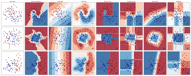
This useful graph below is the best in illustrating this concept. Check from sklearn documentation for reproducibility. It shows the performance of different algorithms for different data sets.

Take a moment to grasp this graph because it reveals a lot about every algorithm. For example:
- Nearest Neighbour Algorithms (KNN) is heavily relying on the closeness of points.
- Linear SVM is trying to slice the data to decide the class of each data point.
- RBF SVM is like KNN in finding linear combinations that separate the data but not in the way KNN does.
- Decision Tree is tackling the problem differently. It is just to do some splits in the data to separate between the classes.
- RandomForest is adopting the same strategy of Decision Tree but with more splits.
- Neural Networks are also trying to get a linear combination of the data to separate classes.
- AdaBoost is also adopting the idea of splits but in an enhanced and modified way.
Based on these observations, let’s try to categorize our algorithms now.
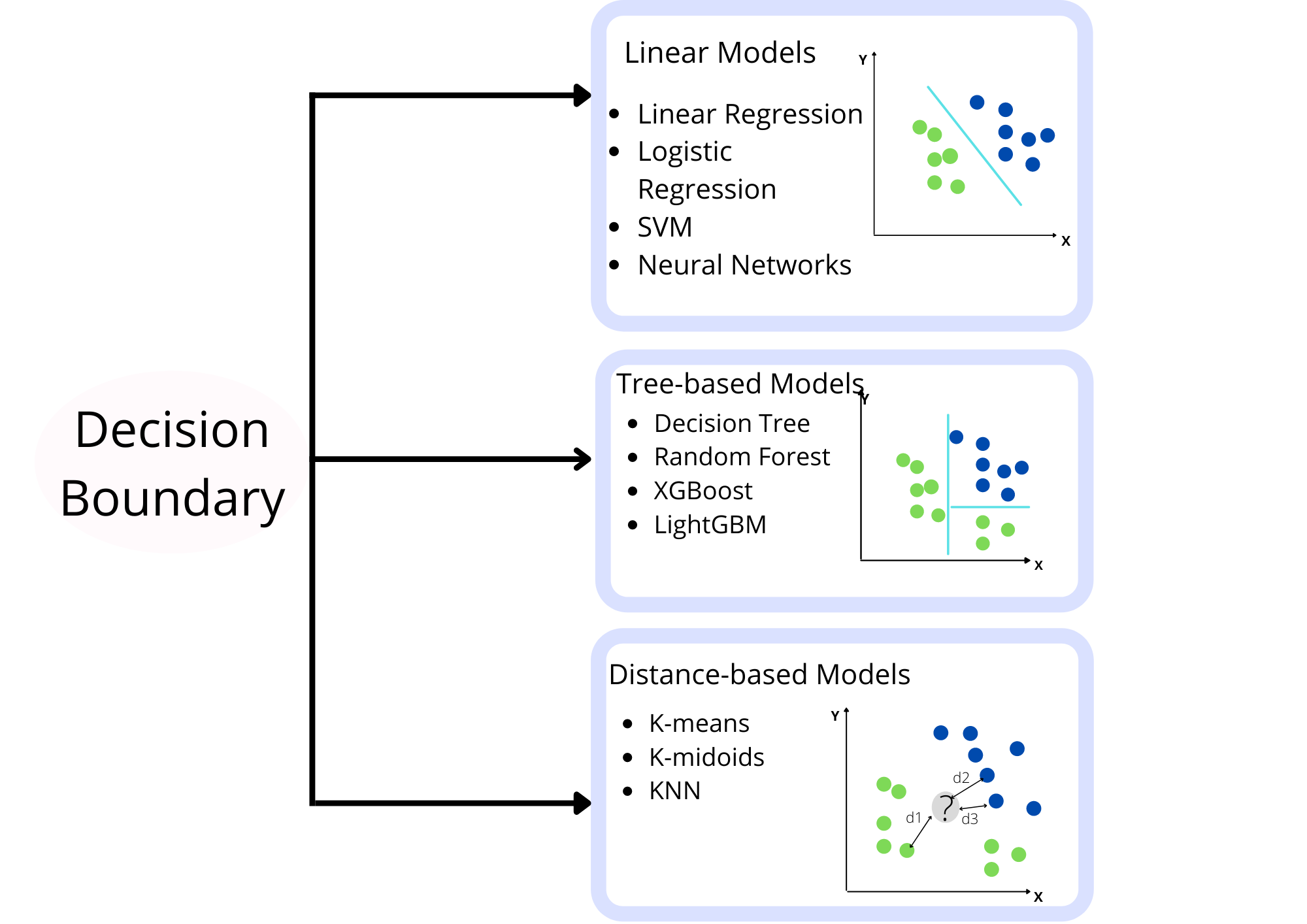
Linear Models
The term linear model implies that the model is specified as a linear combination of features. Based on training data, the learning process computes one weight for each feature to form a model that can predict or estimate the target value.

This category includes the following algorithms:
- Linear Regression
- Logistic Regression
- SVM
- Neural Networks
Tree-based Models
Tree-based models use a series of if-then rules to generate predictions from one or more decision trees. This is also what causes this splitting effect that you can easily see in the above graph.

This category includes the following algorithms:
- Decision Tree
- Random Forest (ensemble methods)
- XGBoost (ensemble methods)
- LightGBM (ensemble methods)
- GradientBoosting (ensemble methods)
- AdaBoost (ensemble methods)
- CatBoost (ensemble methods)
Distance-based Models
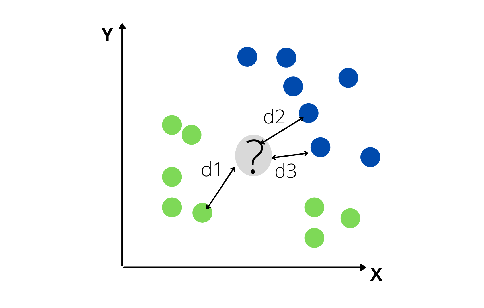
Distance-based models rely on determining the decision boundary based on the closeness of the points to each other. So, they are profoundly affected by the scale of each feature.

Based on the previous categorization, we can turn our question to a simpler one. Are the features in our data helpful for the idea of splits, so we should pick one of the tree-based models? Or are they more useful in creating linear trends between the features and the target so we should choose a linear model?
Now, what should we do to answer these questions?

Exploratory Data Analysis (EDA)
The ultimate goal of the EDA process is to know, explore, and visualize your data. Also, after understanding the data, EDA should help in deciding the best algorithm for your data. Maybe EDA’s process has no clear steps to do, but we can do a little summarization of this process. Besides, we will comment on how each step can reveal a piece of info about the best algorithm to use.
1- Look at Summary statistics and visualizations
- Percentiles, ranges, variance, and standard deviation can help identify the range for most of the data.
- Averages and medians can describe the central tendency.
- Correlations can indicate strong relationships.
2- Visualize the data
- Box plots can identify outliers.
- Density plots and histograms show the spread of data.
- Scatter plots can describe bivariate relationships.
Now, let’s comment about how the outcomes of these two steps will contribute to model selection.
Outliers
Lots of the above statistics and measures will denote information about the dispersion of our data. Keep in mind that lots of outliers will affect any linear model you choose, as the model will try to fit the points with high weights. This should make you think about the following questions.
- Would a linear model help with the existence of these outliers?
- If the outliers’ problem persists, What is the best way to handle them, and what is the handling method that will serve our model of choice?
Normality
The above measures and graphs show the distribution of our data and the correlation between features and the target variable. This should make you think about another two critical things
-
Lack of data normality may add a point in using a tree-based model as the idea of splits is less affected by the data normality.
-
The strong correlation will add a point in using a linear model as it makes it easier for a model to construct some sort of linear combination boundaries. On the other hand, using a tree-based model will be less affected by the weak correlation.
Missing Values
The information denoted about the missing values should ignite some thoughts in every data scientist’s mind. For example,
- Are the missing values related to some specific event, so they should be treated as a separate category of data? Consequently, they will be more beneficial to a tree-based model?
- If the need for a linear model persists, what is the best imputation technique that will make these values of a considerable effect on our model?
- Will using a model that can handle the missing values internally like Naive Bayes or XGBoost alleviate the problem? (Note: sklearn implementation for Naive Bayes algorithm does not allow missing values, but you can implement it manually)
Feature Engineering
After the process of EDA, you must have thoughts about the model of choice. At least you are more inclined to model family over another. Now, the process of feature engineering should be done with respect to some model family. Let’s see some of the standard procedures in feature engineering and how they affect the model performance.
Missing Values Handling
- Imputing the missing values with the “Unknown” category when dealing with categorical variables will be more beneficial to tree-based models.
- Imputing the missing values with the mean or median will be more beneficial to linear models over tree-based models.
- Models that can handle missing values can be susceptible, and not handled missing values can lead them to more reduced performance.
Outliers Handling
- Clipping can be with more value to any linear model as it increases the data normality, but it causes some information loss.
- Transformations like logarithmic or square root transformation can add a damping effect to the values without any information loss. So, it’s more beneficial to linear models.
- Tree-based models are less affected by outliers in general because the idea of splits in them will most probably assign them to a separate split.
Scaling and normalization
- Feature Scaling or normalization has no value when it comes to the tree-based models. That’s because the idea of splits will not be affected by whatever the scale of the data is.
- Normalization is an excellent approach when dealing with linear models. It will lead to faster training and better scores.
- Distance-based models are profoundly affected by the scale of the features. This will open up a door to enforce one feature over another just by increasing its scale.
Categorical Variables Handling
- Some approaches, like One-hot encoding and frequency encoding, can be of great help to a linear model.
- On reversal, approaches like label encoding are beneficial to a tree-based model as they will boost the ability of a model to do data splits.
After sharing some thoughts in the process of EDA and feature engineering, that will make us more oriented to the best model that can fit our problem. Let’s talk more about non-data related considerations that may affect our choice of the model.
Deployment Considerations
In the next few lines, we will ask questions related to our model of choice but not the data itself. For example:
- What is your data storage capacity? Depending on your system’s storage capacity, you might not be able to store gigabytes of classification/regression models or gigabytes of data to train on.
- Does the prediction have to be fast? In real-time applications, it is essential to have a prediction as quickly as possible. For instance, in autonomous driving, road signs must be classified as fast as possible to avoid accidents.
- Does the learning and training process have to be fast? In some circumstances, training models quickly is necessary: sometimes, you need to rapidly update, on the fly, your model with a different dataset.
Usability Considerations
Now, as we have discussed various families of models, best practices in EDA and feature engineering should be done with respect to a model family, and addressed some deployment considerations that may outweigh the use of one model over another. We will now discuss a crucial aspect of any model that every data scientist should be aware of.
Explainability Vs. Predictability
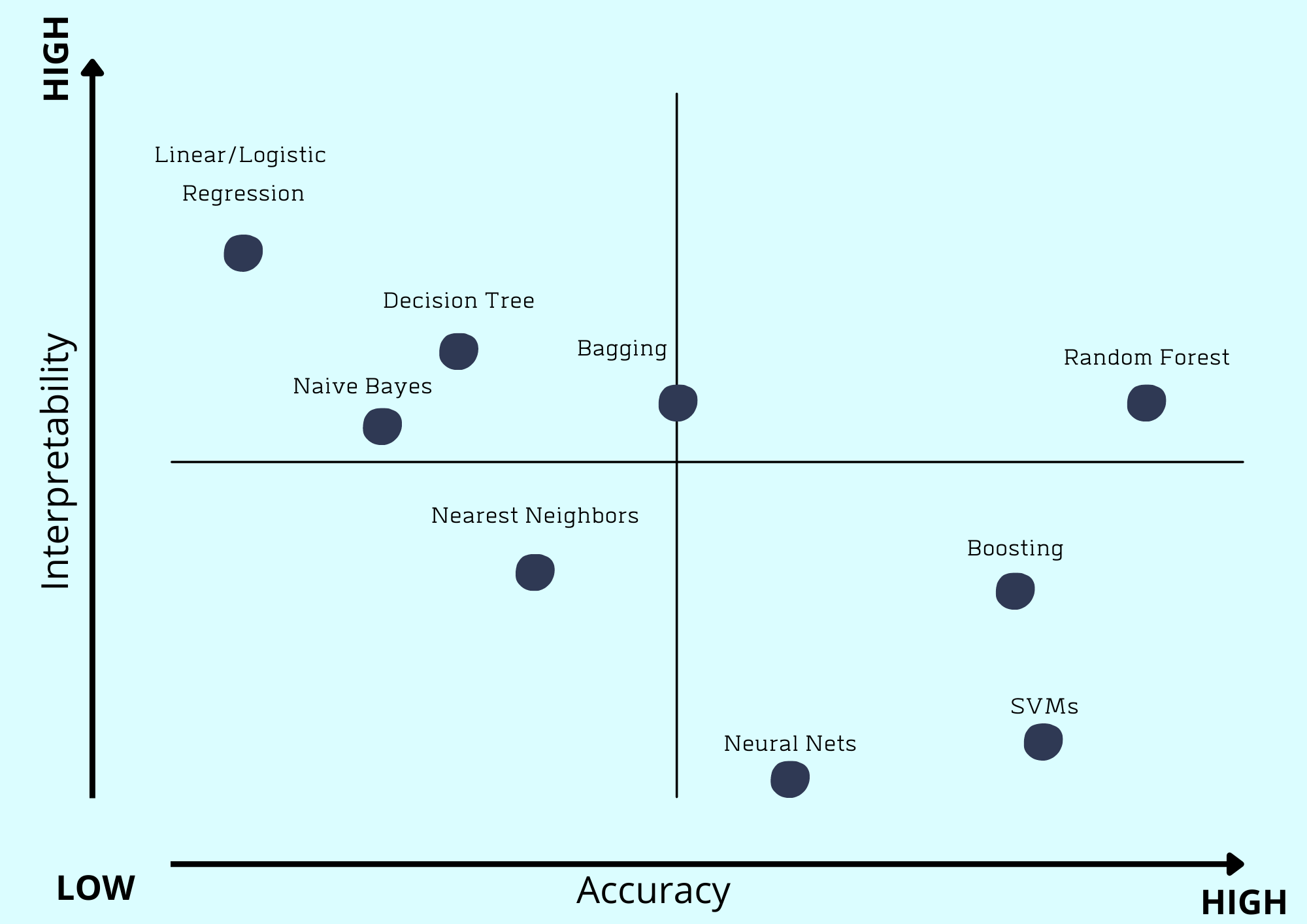
- Explainability means how much you could explain your model prediction. For example, Decision Tree is a very explainable model. Once you have a prediction from it, you can quickly tell you why you get this prediction by following the series of splits (if-then rules). These models are often called white-box models.
- Predictability means what is the predictive power of your algorithm, regardless of the ability to know why it gives a specific prediction for some input. For example, Neural Network is very complex to understand why it provides a particular prediction. These models are often called black-box models.
Sometimes you must be aware of this trade-off as the application may require some explainability in your models of choice, so you will end up using simpler models or on reversal. You may not need any explainability for your application. Hence, you may prefer a model with high predictability over a simpler one. Below is a graph that shows this trade-off for various machine learning algorithms.
